Laminar flow around cylinder
This tutorial explains how to create a simulation case in local computer by using GUI of Code_Saturne, and submit it to the VILJE system.
Setting up the case
The first thing to do before running Code_Saturne is to prepare the computation directories. In this example, the study directory cylinder/ will be created, containing a single calculation sub-directory case1. This is done by typing the command:
$ code saturne create -s cylinder -c case1
The mesh files (circle_cylinder.neu and/or fluent.cgns) files should be copied in the directory MESH/ . ‘circle_cylinder.neu’ is in the Gambit neutral format. ‘fluent.cgns’ is the same mesh in CGNS format which is created by ANSYS mesher. The Code_Saturne Graphic User Interface (GUI) is launched by typing the following command lines:
$ cd cylinder/case1/DATA
$ ./SaturneGUI &
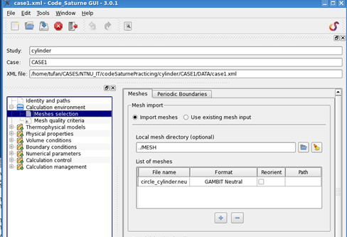
After launching the GUI, The mesh files should be added in mesh selection part by pressing ‘+’ as seen in the Figure.
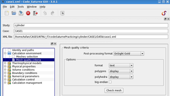
At the next section: Mesh quality criteria, clicking ‘Check mesh’ button gives some information about the solution grid and shows the failures if there is any problem.
Next section, the unsteady flow should be selected. The flow around cylinder will be calculated by unsteady algorithm.
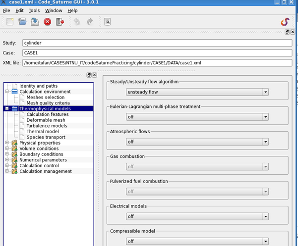
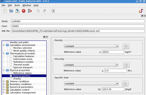
At the Thermophysical models part, laminar flow should be selected. There is no thermal model in the flow because there is no heat transfer will be calculated. Thus, the other options should be default ones. ‘Physical properties’ is the place where Reynolds number is defined. The density and viscosity should be defined here (1000 kg/m3 and 1 Pa.s)
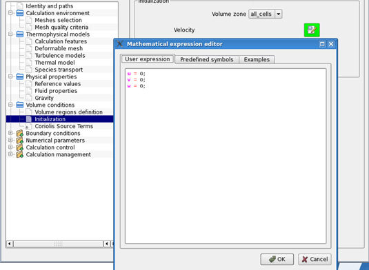
Initial values should be defined at the popping screen by clicking the green bottom at the ‘Initialization’ part. In this case, all initial velocity components are zero.
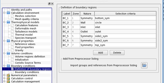
Boundary conditions can be loaded by clicking the button at the section of ‘Add from Preprocessor listing’. If there is an error or missing zone, the boundary conditions can be applied manually by pressing ‘Add’ button and selecting proper type of b.c for each surface or cell zone.
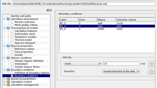
At the next section, the parameters of each boundary should be applied separately. For example the inlet velocity should be specified at the inlet boundary condition (incoming flow velocity is 1 m/s). There is nothing to apply at the outlet and the wall b.c. in this case. Default options will stay.
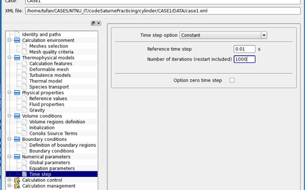
At the ‘Numerical Parameters’ section, Global parameters and Equation parameters can be stayed at default options for this example. Time step option should be adjust to 0.01 seconds. Enter the number of iterations necessarily to reach fully developed flow field (for this example, 1000 is used as seen in the Figure).
Remember to save the xml file at regular intervals during this tutorial changes.
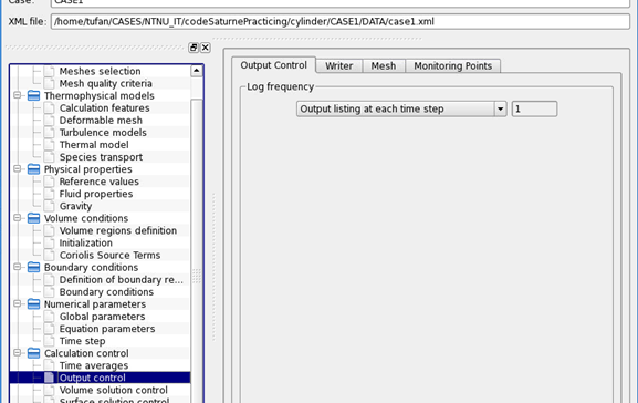
At the calculation part, ‘Time averages’ part is for to record time averaged fields during simulation. Mean velocity field can be calculated here. ‘Output control’ has 4 tabs. The first one is the controlling the frequency of written information to listing file (Code_Saturne’ s output). At the Write tab, the default output is Ensight format. The format can be adjusted or more writers can be added with different other formats by clicking ‘+’ button.
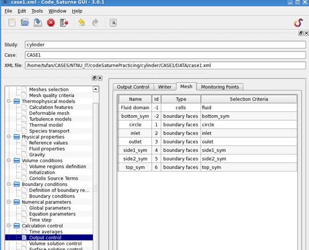
At the ‘Mesh’ tab, the name and the type of the boundary faces, cells should be specified and assigned to a ‘Writer’ which is defined before. In this way the boundary surfaces can be appeared in the postprocessing.
The rest of the parameters will not be touched in this example. In the performance tuning part, more options for the calculations can be set up. The partitioning method, MPI-IO options can be selected based on the configuration options selected during the compilation of the Code_Saturne.
Save the xml file from GUI and exit.
Preparing the job script
Now you move to case folder by typing:
$ cd ..
It is necessary to write following commands to create a solver script based on the case1.xml parameter file created before. Code_Saturne should be either loaded as a module or defined in the bashrc file as an environment for individual compilations. Intel compiler and MPT (versions used for Code_Saturne is built) should be loaded beforehand:
$ module load intelcomp/2.06 mpt/13.0.1
$ code saturne run --initialize --param case1.xml
Now there is a folder created in the RESULT/ with a name indicating the date and time that you initiated the case with that command. There is one script file named run_solver.sh created in this folder. This script file is normally created for a serial run. It should be modified to submit to the VILJE with batch system and run the case in parallel. Here is an example (64 cores) for the modified run_solver.sh file. The red lines are the added to the original file.
#!/bin/bash
#-------------------------------------------------------------------
#PBS -N CS_128
#PBS -l select=4:ncpus=32:mpiprocs=16:ompthreads=1
#PBS -l walltime=1:00:00
#PBS -A nn9191k
#PBS -j oe
#-------------------------------------------------------------------
# Detect and handle running under SALOME YACS module.
YACS_ARG=
if test "$SALOME_CONTAINERNAME" != "" -a "$CFDRUN_ROOT_DIR" != "" ; then
YACS_ARG="--yacs-module=${CFDRUN_ROOT_DIR}"/lib/salome/libCFD_RunExelib.so
fi
module purge
module load mpt/2.06
module load intelcomp/13.0.1
# Export paths here if necessary or recommended.
cd /home/ntnu/<user>/CASES/NTNU_IT/CS/roundCorner/pert0.1/RESU/20140213-2100
# Run solver.
mpiexec_mpt -np 64 /home/ntnu/<user>/code_saturne/intel_tau_noPapi/ptscotch/mk_hd_cg_io_omp/target_v3.0.1/libexec/code_saturne/cs_solver --param case1.xml --mpi $YACS_ARGS $@
export CS_RET=$?
exit $CS_RET
Running the job with the script
Submit the job by command:
$ qsub RESU/<date and time>/run_solver.sh
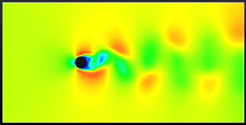
During the simulations, the output can be tracked from ‘listing’ file in the RESU/****/ folder with ‘tail -f’ command. After the job is successfully finished, the results are written In the RESU/****/postprocessing folder. ‘Results.case’ file is an Ensight file but can be open with Paraview. An example picture from the results can be seen in the next figure.