Allinea Performance Reports
Allinea Performance Reports is a performance evaluation tool that as result produces a single HTML page with a characterisation of the problems that the evaluated program has. It divides the characterization into the categories CPU, MPI, I/O, and memory and it produces evaluations like: "The per-core performance is memory-bound" and "Little time is spent in vectorized instructions".
Load the module
Allinea Performance Reports needs to compile a library that is pre-loaded before you program is run. In order to compile this library, the Intel compiler and the MPT library must be loaded as well, regardless of whether the program to be evaluated has been compiled with the Intel compiler:
$ module load intelcomp/16.0.1 mpt/2.14 python/2.7.12 perf-reports/6.1.2
Remember that you must also load these modules in job scripts, when you run your program.
Compile your program
When you compile your program then you must compile it with MPT 2.13. You should use optimizations flag like -O2, -O3 and -xAVX, because Allinea Performance Reports then will be able to tell you if your program manages to use vectorized instructions. You must also link with the Allinea libraries, such as in:
make-profiler-libraries
ifort -o rank rank.f90 -L$PWD -lmap-sampler-pmpi -lmap-sampler -Wl,--eh-frame-hdr -Wl,-rpath=$PWD -lmpi
Analysing your program on login nodes
If your program only runs for a short while using few processes, then you can analyze it while running it on a login node:
perf-report mpirun -np 4 rank
After your program has run, you can find the produced performance report in an HTML file with a name similar to interFoam_4p_2014-06-20_13-34.html. Copy this file to your local pc and view it there.
Analysing your program in batch jobs
In batch jobs, you must call your program with:
perf-report mpiexec_mpt rank
where you explicitly write the number of processes that your program runs on. After your program has run, you can find the produced performance report in an HTML file with a name similar to rank_4p_2014-06-20_13-34.html. Copy this file to your local pc and view it there.
Allinea MAP
Allinea MAP is a performance evaluation tool that uses a GUI for presenting the performance of a program. It presents the execution of a program as a number of horizontal graphs. It is possible to select the metrics that the graphs are based on. By click-and-drag on the graphs, one can select a small part of the execution time. At the bottom of the GUI, one can then see the code that was running in that period.
Load the module
Allinea MAP needs to compile a library that is pre-loaded before you program is run. In order to compile this library, the Intel compiler and the MPT library must be loaded as well, regardless of whether the program to be evaluated has been compiled with the Intel compiler:
$ module load intelcomp/16.0.1 mpt/2.14 python/2.7.12 perf-reports/6.1.2
Remember that you must also load these modules in job scripts, when you run your program.
Compile your program
When you compile your program then you must compile it with MPT 2.14. You must compile your program with the -g flag and you should use a low level of optimization, such as -O0 or -O2, to avoid that the assembler code becomes too different from the source code, because Allinea MAP will tell you what lines in your source code that takes up most of the time. You must also link with the Allinea libraries, such as in:
make-profiler-libraries
ifort -o rank rank.f90 -L$PWD -lmap-sampler-pmpi -lmap-sampler -Wl,--eh-frame-hdr -Wl,-rpath=$PWD -lmpi
Create a job-script template file
In order to submit jobs to the queue using the GUI, you must show Allinea MAP how a job script for Vilje looks like. You do that by creating a general job script template and then telling Allinea MAP where this template file is. This is an example of a template file:
#!/bin/bash
# Name: PBS SGI MPT
# Use with SGI MPT (Batch)
#
# WARNING: If you install a new version of Allinea Forge to the same
#          directory as this installation, then this file will be overwritten.
#          If you customize this script at all, please rename it.
#
# submit: qsub
# display: qstat
# job regexp: (\d+.service2)
# cancel: qdel JOB_ID_TAG
# show num_nodes: yes
#
# WALL_CLOCK_LIMIT_TAG: {type=text,label="Wall Clock Limit",default="00:30:00",mask="09:09:09"}
# QUEUE_TAG: {type=text,label="Queue",default=debug}

## Allinea Forge will generate a submission script by
## replacing these tags:
##        TAG NAME         |         DESCRIPTION           |        EXAMPLE
## ---------------------------------------------------------------------------
## PROGRAM_TAG             | target path and filename      | /users/ned/a.out
## PROGRAM_ARGUMENTS_TAG   | arguments to target program   | -myarg myval
## NUM_PROCS_TAG           | total number of processes     | 16
## NUM_NODES_TAG           | number of compute nodes       | 8
## PROCS_PER_NODE_TAG      | processes per node            | 2
## NUM_THREADS_TAG         | OpenMP threads per process    | 4
## DDT_DEBUGGER_ARGUMENTS_TAG | arguments to be passed to ddt-debugger
## MPIRUN_TAG              | name of mpirun executable     | mpirun
## AUTO_MPI_ARGUMENTS_TAG  | mpirun arguments              | -np 4
## EXTRA_MPI_ARGUMENTS_TAG | extra mpirun arguments        | -x FAST=1

#PBS -N Job_name
#PBS -l select=NUM_NODES_TAG:ncpus=32:mpiprocs=PROCS_PER_NODE_TAG
#PBS -l walltime=WALL_CLOCK_LIMIT_TAG
#PBS -o PROGRAM_TAG-allinea.stdout
#PBS -e PROGRAM_TAG-allinea.stderr
#PBS -q test
#PBS -A Account_name

module load intelcomp/16.0.1
module load mpt/2.14
module load python/2.7.12
module load forge/6.1

cd $PBS_O_WORKDIR
export OMP_NUM_THREADS=1

DEBUGGER_OPTIONS="DDT_DEBUGGER_ARGUMENTS_TAG" mpiexec_mpt AUTO_MPI_ARGUMENTS_TAG PROGRAM_TAG PROGRAM_ARGUMENTS_TAG
You must change Job_name and Account_name. You must also, of course, add any special setup commands that your program requires.
Notice the line:
#PBS -q test
There are, at the time of writing, only 4 compute nodes that are dedicated to the test queue and the max. wall time is 1 hour. There are also, at the time of writing, only 64 licenses in total for Allinea MAP, so with 16 processes on each compute node, you can at max. use 4 compute nodes.
The following line:
export OMP_NUM_THREADS=1
is to compensate for a bug that Allinea MAP has, at the time of writing. If one does not need OpenMP and therefore disable it on the GUI, then PBS will still set OMP_NUM_THREADS to 32. The software, that is run in batch, only uses this value to determine if the sampling rate should be reduced, to avoid getting too much sampling data. So if one profiles a program that does not use OpenMP, then the sampling rate will needlessly be reduced, because of the value of OMP_NUM_THREADS. If your program actually is OpenMP parallelized, then you must delete this line.
Analysing your program in batch
Start Allinea MAP:
$ module purge
$ module load intelcomp/16.0.1 mpt/2.14 python/2.7.12 forge/6.1.2
$ map <<program name>>
When you have the GUI, then do the following:
1. set "Working Directory"
2. select "MPI" and view details
3. Select "Submit to Queue".
3.1 Click "Configure". Choose the file "pbs-sgi-mpt.qtf" as your
Submission template file.
3.2 Click "Ok".
3.3 Click "Paramters"
3.4 Set the wall clock limit.
3.5 set the queue to "test"
4. Link the "Number of Processes" and "Number of Nodes" together.
5. Set the processes per node to 16
6. Change the number of nodes 2
7. Change the Implementation to "SGI MPT (2.10+, batch)".
8. Deselect "OpenMP"
9. Click "Submit".
10. Click "Go".
Examining the results
The first thing that you must do is to choose the right metrics. On right, under the horizontal graph at the top, there is a button for selecting the viewed metrics. If you, for instance, are interested in the performance of the MPI calls in your program, then you click this button and select "Preset MPI". When you have the right metrics selected, then you choose a part of a graph to examine in further detail. Find a part on of the graphs that looks interesting. Then left-click right before this interesting part, drag to the other side of it, and then release. Thereby you will have the highlighted the interesting part on the graph. At the bottom of the GUI you are now able to find the lines in your code that was responsible for the activity that you selected on the graph.
TAU
TAU is a performance evaluation tool that supports parallel profiling and tracing. TAU provides a suite of static and dynamic tools that provide graphical user interaction and inter-operation to form an integrated analysis environment for parallel Fortran, C++, C, Java, and Python applications. Profiling shows how much (total) time was spent in each routine, and tracing shows when the events take place in each process along a timeline. Profiling and tracing can measure time as well as hardware performance counters from the CPU.
Instrument your program
-
Set the proper environment by loading the TAU modulefile, e.g.
$ module load tau
-
TAU provides wrapper scripts, tau_f90.sh, tau_cc.sh and tau_cxx.sh to instrument and compile Fortran, C, and C++ programs respectively. E.g. edit your Makefile as follow
CC  = tau_cc.sh
CXX = tau_cxx.sh
F90 = tau_f90.sh
and compile your program. This will result in an instrumented executable that automatically calls the Tau library to record the values of performance registers during program execution. Run the program.
-
At job completion you should have a set of profile.* files. These files can be packed into a single file with the command:
$ paraprof --pack app.ppk
Analysis
-
Launch the
paraprofvisualization tool together with the profile data file:$ paraprof app.ppk
Two windows will appear, the ParaProf Manager Window and the Main Data Window.
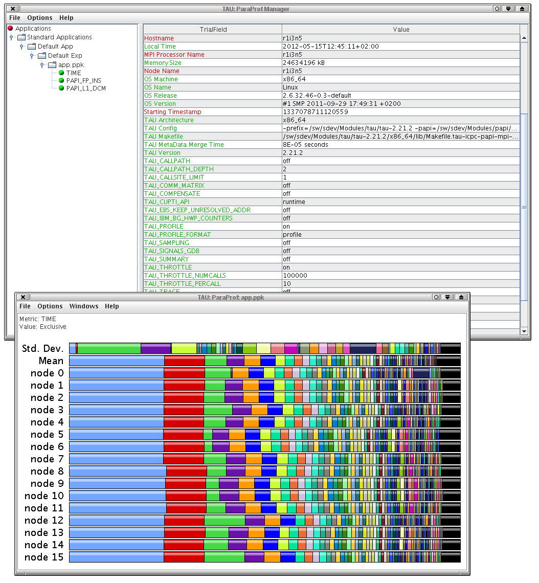
Figure 1. ParaProf manager and main data windows
(Click to enlarge) - The Main Data Window shows where the program used most time. The longer the bar, the more time was spent in this part of the code.
- Right-click on the longest bar and select Show Source Code. This will show a file where one of the functions is highlighted in blue. This function is where your program spends most of its time.
-
Get more detailed information of the function found in the previous step. Exit paraprof and create a file named select.tau in the source code directory with the following content:
BEGIN_INSTRUMENT_SECTION
loops routine="#"
END_INSTRUMENT_SECTION
-
Type at the command line:
$ export TAU_OPTIONS="-optTauSelectFile=select.tau -optVerbose"
Delete the object file (*.o) of the source code file containing the function found earlier. Recompile the code and rerun the executable.
Viewing the new profile data file withparaprofas before, in the source code only the single loop where most time is spent is highlighted, instead of the entire function.

Using Hardware Counters for Measurement
-
For example, to analyse the code for floating-point operations versus cache misses ratio, set the environment variable TAU_METRICS:
$ export TAU_METRICS=TIME:PAPI_FP_INS:PAPI_L1_DCM
Delete the profile.* files and rerun the program. This will result in three multi_* directories.
- Pack and view the results as before.
- In the ParaProf Manager Window choose Options → Show derived Metric Panel
- In the Expression panel click to make the derived metric "PAPI_FP_INS"/"TIME". Click apply.
- Double-click this new metric listed. In the window that appears find the text node 0 and single-click it. A new window appears listing values for the floating-point operations versus cache misses ratio.
You can now consider how to change your program, e.g. changing the order of the loops, in order to make the ratio between floating point operations and cache misses go up. Once you have made a change, recompile your program and repeat the process listed above.
Further Information
- For more information see the online TAU Documentaion
Open|SpeedShop
Compile your code with debugging enabled (-g). Load the Open|SpeedShop module:
$ module load openspeedshop
To use Open|SpeedShop with an MPI program, call the relevant command with the original statement in quotation marks. For example:
$ osspcsamp "mpirun -np 4 myprog arg1 arg2"
The resulting 'myprog-pcsamp.openss' file can then be viewed with the command:
$ openss -f myprog-pcsamp.openss
Further Information
- For more information, read this article.
Scalasca
Scalasca is a software tool that supports the performance optimization of parallel programs by measuring and analyzing their runtime behavior. The analysis identifies potential performance bottlenecks – in particular those concerning communication and synchronization – and offers guidance in exploring their causes.
Instrument your program
-
Set the proper environment by loading the Scalasca modulefile, e.g.:
$ module load intelcomp/15.0.1 mpt/2.11 scalasca/2.2
-
Scalasca does not itself provide a special command or wrapper script for instrumentation of the code. Instead, it uses the Score-P program. Edit your makefile and change CC, CXX and FF to:
CC  = scorep icc
CXX = scorep icpc
FF  = scorep ifort
and re-compile your program. This will result in an instrumented executable that automatically calls the Score-P library to record the values of performance registers during program execution. Score-P is and individual performance analysis tool that you can read about here.
-
Set the name of the directory where you want the data to be stored, e.g.:
$ export SCOREP_EXPERIMENT_DIRECTORY=name-of-directory
This must also be set in batch job scripts. After you have done this, you run your program, prepending
scalasca -analyzeto your program, e.g.:$ scalasca -analyze mpirun -np 4 ./name-of-program
At job completion you should have a directory with the name that you chose. Notice, that if you are running in batch and therefore usually would use the command:
mpiexec_mpt ./name-of-program
in your batch script, then you cannot just put
scalasca –analyzein front of this command. The reason for this is that scalasca does not know the number of MPI processes that your program is running on and.therefore looks at the options tompiexec_mptto get this information. You must therefore provide this information with the-npoption, such as in:scalasca -analyze mpiexec_mpt -np 144 ./name-of-program
Analysis
Launch the Scalasca visualization tool together with the profile data:
$ scalasca -examine name-of-directory
A window then appears, where you in the left when can select the metric that you want to use, in the middle window examine the call tree for the selected metric and in the right window view the system tree:

Figure 2. Scalasca main data window
(Click to enlarge)
If you right-click on the blue line in the middle "Call tree" then you get menu where one of the options is "Called region". Selecting this option opens up a sub-menu where one of the options is "Source code". Click on this option to view the corresponding source code.